Written Tutorial

'use strict';
 
const admin = require('/MarkLogic/admin.xqy');
const config = admin.getConfiguration()
const groupid = admin.groupGetId(config, "Default")
const odbc = admin.odbcServerCreate(config, groupid, "5432-geo-odbc", "/", 5432, 0, xdmp.database("Documents") )
admin.saveConfiguration(odbc);

Create query-based views

If you haven’t already, insert some data and a view by running steps labeled Example Document: Single City , Example Document: Multiple Cities, and TDE Template for a View called "Towns"

A known limitation of many of the GIS tools is that there must only be ONE geometry column per view and ONE integer ‘id’ primary key column to achieve fully expected results. So, let’s create some query-based views (QBV) to work around this limitation.

You must have the query-view-admin role to insert a query-based view. If you created a new Schemas database for this tutorial, substitute the four instances of Schemas in the calls to xdmp.eval() below for your Schemas database.

'use strict';
const op = require('/MarkLogic/optic');
 
const view0 = op.fromView('regions','towns')
               .select([op.col('geoid'), op.col('interiorPoint')])
               .generateView('Towns', 'PointView')
 
xdmp.eval('declareUpdate(); \
          xdmp.documentInsert("pointQBV.xml", view, \
          {collections: "http://marklogic.com/xdmp/qbv"})', {view: view0},
        { database: xdmp.database('Schemas') });
 
const view1 = op.fromView('regions','towns')
                .select([op.col('geoid'), op.col('highway')])
                .generateView('Towns', 'LinestringView')
 
xdmp.eval('declareUpdate(); \
          xdmp.documentInsert("linestringQBV.xml", view, \
          {collections: "http://marklogic.com/xdmp/qbv"})', {view: view1},
        { database: xdmp.database('Schemas') });
 
const view2ColDescription =
[
 {
   "name": "tenKmRadiusPolygon",
   "type": "polygon",
   "invalid-values": "reject",
   "coordinate-system": "wgs84"
 }
]
const view2 = op.fromView('regions','towns')
                .bind(op.as('tenKmRadiusPolygon', op.geo.circlePolygon(op.col('tenKmRadius'), 0.05)))
                .select([op.col('geoid'), op.col('tenKmRadiusPolygon')])
                .generateView('Towns', 'CirclePolygonView', view2ColDescription)
 
xdmp.eval('declareUpdate(); \
          xdmp.documentInsert("circlePolygonQBV.xml", view, \
          {collections: "http://marklogic.com/xdmp/qbv"})', {view: view2},
        { database: xdmp.database('Schemas') });
 
const view3 = op.fromView('regions','towns')
                .select([op.col('geoid'), op.col('exactGeometry')])
                .generateView('Towns', 'polygonView')
 
xdmp.eval('declareUpdate(); \
          xdmp.documentInsert("polygonQBV.xml", view, \
          {collections: "http://marklogic.com/xdmp/qbv"})', {view: view3},
        { database: xdmp.database('Schemas') });

Notice that in view2, we call op.geo.circlePolygon() on our tenKmRadius circle column and provide a column descriptor to the third argument of its generateView. This is because circles do not have a WKT representation, so we must turn it into an approximate polygon equivalent to pass it over ODBC and be recognizable by QGIS. See Advanced Optic Geo Topics for more QBV tricks.

Let’s see what rows are in each QBV before we put geometries on a map.

'use strict';
let results =
[
xdmp.sql('select * from pointView'),
 
xdmp.sql('select * from linestringView'),
 
xdmp.sql('select * from circlePolygonView'),
   
xdmp.sql('select * from polygonView')
]
 
results;

We successfully created four different views – all with a geoid and a region column – based on our single TDE Towns view. Do not delete or disable this TDE view, or else the four QBVs that depend on it will break.

Connect to MarkLogic

Next, let’s create an ODBC data source. I will be using Windows in this example. The steps to create a data source will be different for Linux and Mac. Learn how to install and configure an ODBC driver.

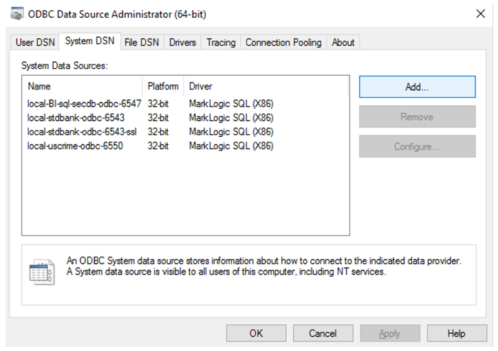
Open the ODBC Data Source Administrator (64-bit). Click on the ‘System DSN’ tab. Click ‘Add…’, choose ‘MarkLogicSQL’ as the driver, and hit ‘Finish’. Enter the relevant information for the ODBC Server.

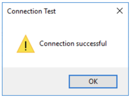
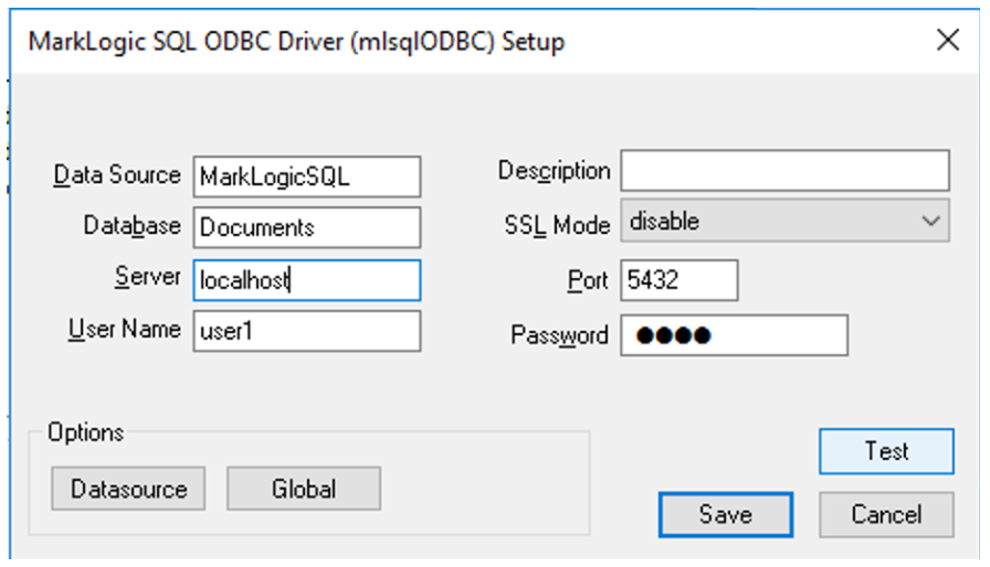Take note of your ‘Data Source’ name, as we will need it in the next steps to connect to QGIS. Test the connection and verify it is successful.

Loading into maps

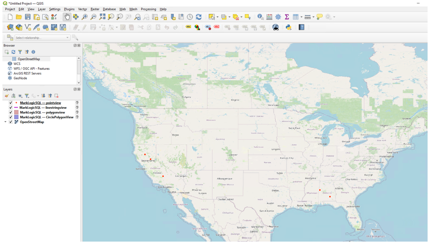
Now, let’s open up QGIS! Start a new project and in the Browser, double-click OpenStreetMap to see a nice map of the world.

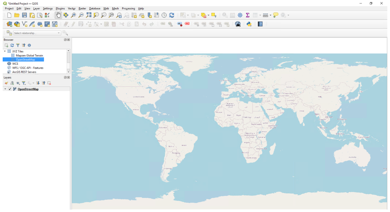
Select EPSG:4326 as the coordinate system (available in the bottom right of the window). This is the spatial reference system ID of wgs84.

Let’s get some of our geometries stored in MarkLogic onto the map.

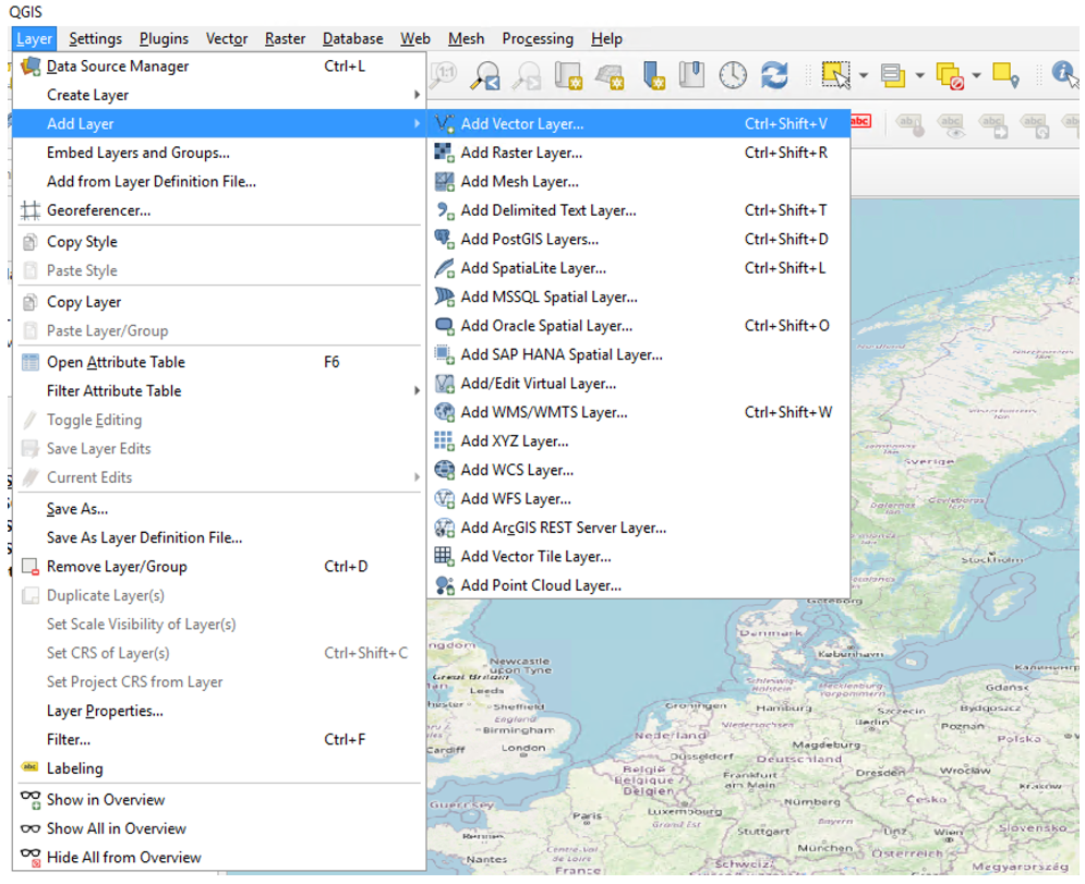
On the menu, Click Layer → Add Layer → Add Vector Layer…

 In the Data Source Manager, click the Database radio button, select type ODBC and hit New.

Fill in the Name and Database fields. Type in the name of the ODBC data source that you configured earlier into the Database field. This is a bit confusing, as ‘Database’ in this case is our ‘Data source’, but such is life.

The rest of the fields will be inferred by the ODBC data source, so we can leave these blank and hit ‘Test Connection.’

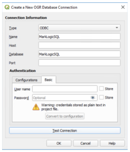
Now that we’ve confirmed our connectivity to MarkLogic through QGIS via ODBC, let’s finally insert those regions. Hit ‘OK’

Make sure we’ve selected the correct connection name, and hit Add.

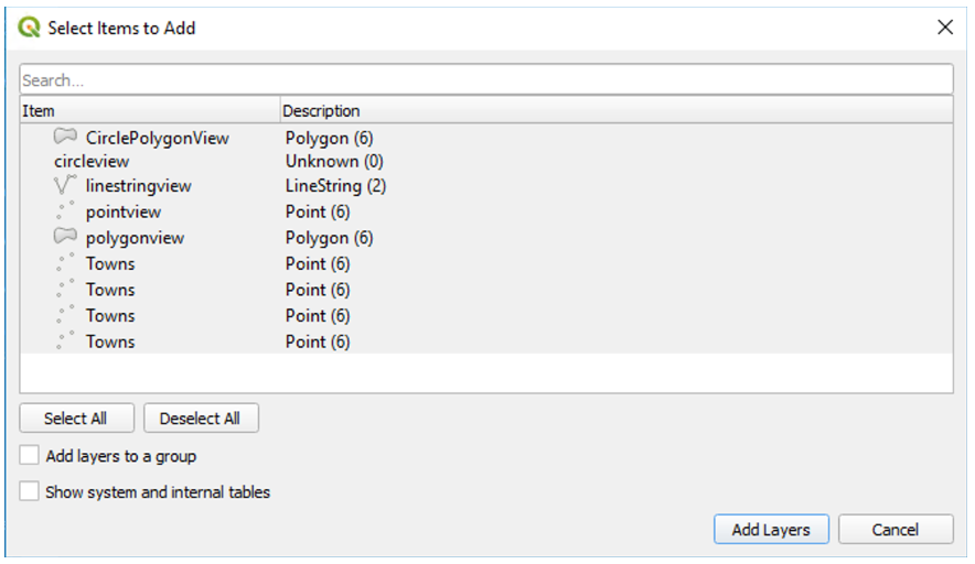Those are our tables! Now we see why we created those QBVs, as Towns communicated that it had 4 geometry columns, but QGIS only recognized the Point column in each.

Shift-click to select all of our QBVs and hit ‘Add Layers’

Let’s move the Layers around in order to see them all. See the order of the Layers from top to bottom in the left pane of the screenshot below, and duplicate this in your QGIS instance (pointview, then linestringview, then polygonview, then CirclePolygonView).

You’re also going to want to decrease the opacity of the polygonview and CirclePolygonView layers for visibility.

Right click on the MarkLogicSQL – polygonview layer → Styles → Edit symbol…

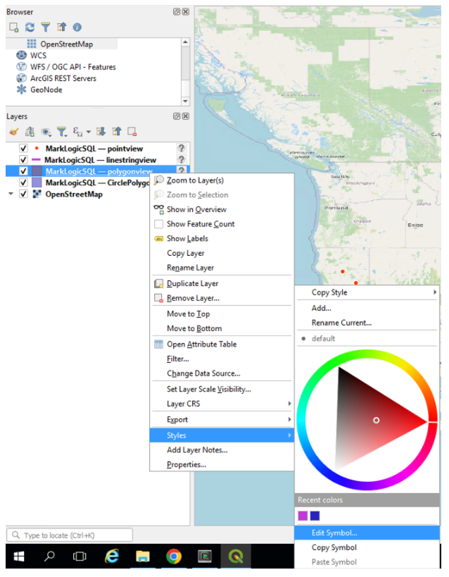Move the Opacity slider to 50% for polygonView and CirclePolygonView. You can also adjust your colors here.

Interacting with geometries

Now, let’s examine our geometries!

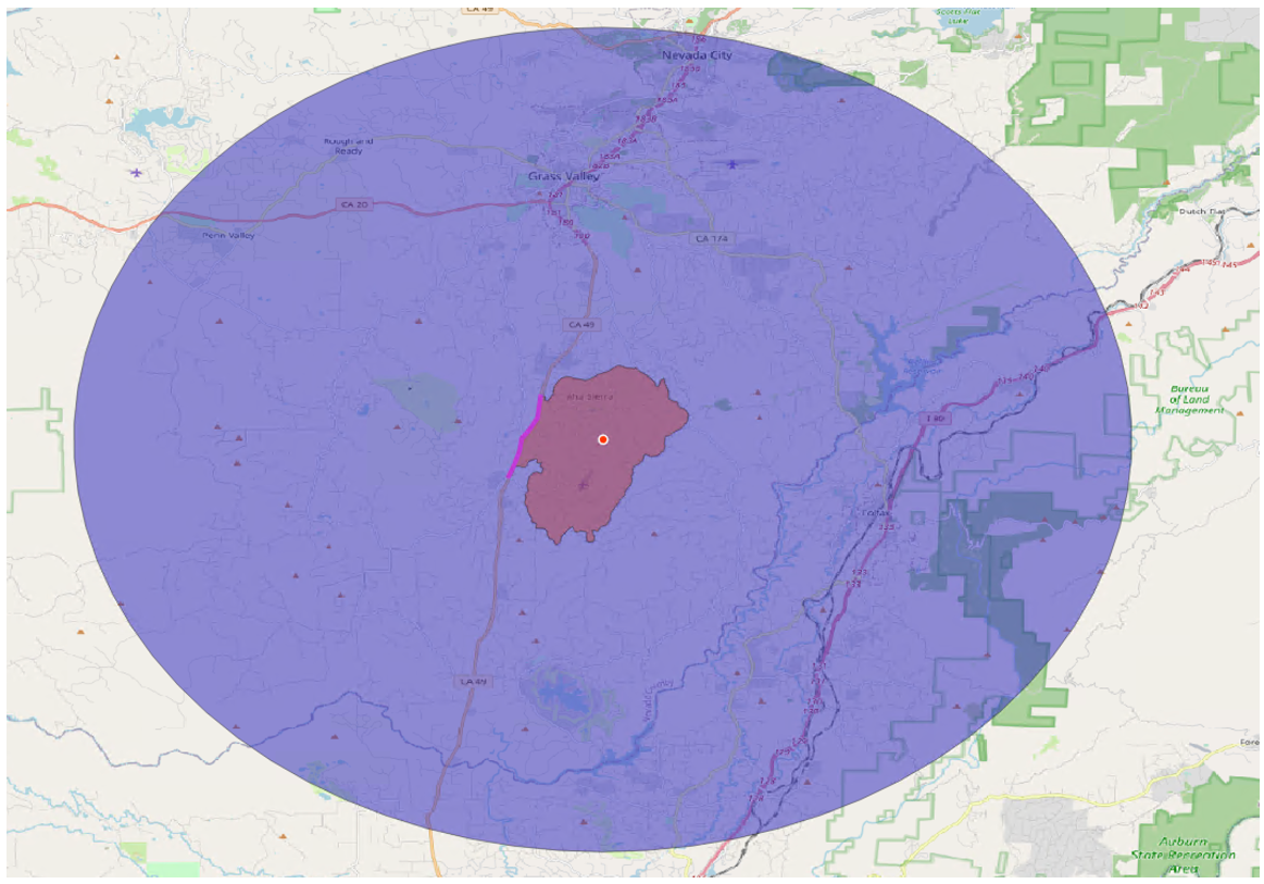Above is a zoomed-in view of the geometries we stored in Alta Sierra, California. Here, we see the highway intersection in pink, the interiorPoint in bright red, the exactGeometry in darker red, and the tenKmRadius in indigo.

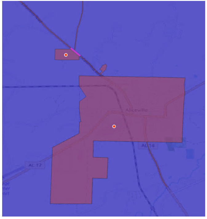
You can also apply filters to your layers to bring the spotlight to the geometries you are interested in. Let’s consider our neighboring Alabama towns McMullen and Aliceville for this example.

Let’s filter out the geometries in the polygonview that don’t CROSS a rough sketch of Highway 14.

Right click MarkLogicSQL – polygonview → Filter…

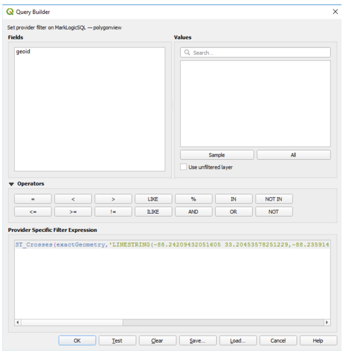
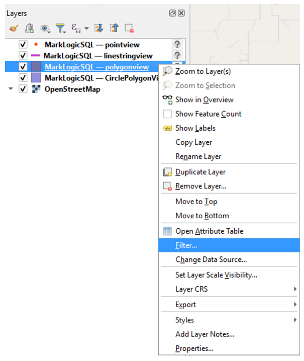In the Filter Expression, we can type valid SQL that will appear in the WHERE clause of a SQL query. This SQL query will be sent to MarkLogic and evaluated, allowing for flexible custom filtering on geometries.

Let’s input this into the Filter expression:

Hit Test, and if the query is valid, we will see that the where clause returned 1 row. Hit OK.

ST_Crosses(exactGeometry,'LINESTRING(-88.24209432051605 33.20453578251229,-88.23591451094573 33.199652135431265,-88.23213796065276 33.194768215944954,-88.22630147383636 33.18701084280127,-88.22218160078948 33.18097685538396,-88.20604543135589 33.17637925271159,-88.19814900801605 33.17350562854858,-88.19162587569183 33.166321155936494,-88.1847594206137 33.16028574390584,-88.17754964278167 33.153675054072735,-88.17171315596526 33.14907601943829,-88.16690663741058 33.144476743690156,-88.16072682784026 33.13872730996478,-88.15317372725433 33.13268999915151,-88.15317372725433 33.12751483080372,-88.14768056319183 33.12665227308664,-88.14905385420745 33.1220518221529,-88.1463072721762 33.11400045308982,-88.14356069014495 33.108536603767405,-88.14115743086761 33.103360012020495)')

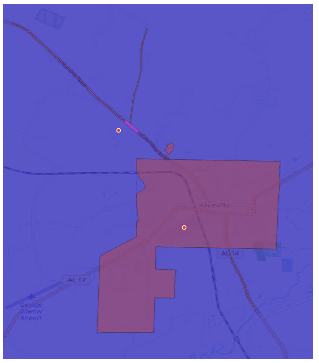
Now, we see that Aliceville is the only town whose exactGeometry satisfies the DE-9IM relation CROSSES with highway 14. Highway 14 does not CROSS McMullen because it does not enter at one point and exit at another point of McMullen’s exactGeometry. Visit the Dimensionally Extended 9-Intersection Model (DE-9IM) wiki page for additional DE-9IM relations.

If we turn on the ODBC ConnectionTask ReceiveMessage trace event in MarkLogic and look in our ODBC ErrorLog, we can see the full queries that are executed.

2022-11-30 13:16:30.162 Info: [Event:id=ODBCConnectionTask ReceiveMessage] => Q SELECT * FROM "polygonview" WHERE ST_Crosses(exactGeometry,'LINESTRING(-88.24209432051605 33.20453578251229,-88.23591451094573 33.199652135431265,-88.23213796065276 33.194768215944954,-88.22630147383636 33.18701084280127,-88.22218160078948 33.18097685538396,-88.20604543135589 33.17637925271159,-88.19814900801605 33.17350562854858,-88.19162587569183 33.166321155936494,-88.1847594206137 33.16028574390584,-88.17754964278167 33.153675054072735,-88.17171315596526 33.14907601943829,-88.16690663741058 33.144476743690156,-88.16072682784026 33.13872730996478,-88.15317372725433 33.13268999915151,-88.15317372725433 33.12751483080372,-88.14768056319183 33.12665227308664,-88.14905385420745 33.1220518221529,-88.1463072721762 33.11400045308982,-88.14356069014495 33.108536603767405,-88.14115743086761 33.103360012020495)')

And that’s it for the basics of how you interact with MarkLogic-stored geometries in QGIS! Hope you found this useful.

Related Resources

• Query Geospatial Data using Optic
• Advanced Optic Geo Topics
• Geo API docs
• Value processing functions
• Dimensionally Extended 9-Intersection Model (DE-9IM)
• Template Driven Extraction (TDE) Chapter of the Application Developer Guide
• Semantics Guide
• Geospatial Chapter of the Search Developer Guide
• Query-based views in the Application Developer Guide
• OGC SQL Spec
• OGC GeoSPARQL Spec